GraphAbs
Create: Normal Q–Q plot anatomy
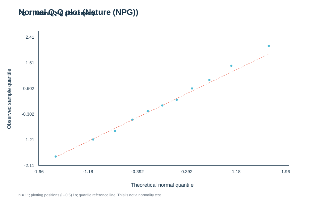
Paste numeric observations, separated by commas or new lines. The plot compares sorted observations with standard-normal quantiles and includes a quartile reference line.
)%22%3E%3Crect%20width%3D%22100%25%22%20height%3D%22100%25%22%20fill%3D%22white%22%2F%3E%3Cstyle%3Etext%7Bfont-family%3AArial%2C%20Helvetica%2C%20sans-serif%3Bfill%3A%2319354a%7D.tick%7Bfont-size%3A14px%7D.label%7Bfont-size%3A17px%7D.small%7Bfont-size%3A12px%3Bfill%3A%2365717d%7D%3C%2Fstyle%3E%3Ctext%20x%3D%2260%22%20y%3D%2248%22%20font-size%3D%2226%22%20font-weight%3D%22700%22%3ENormal%20Q-Q%20plot%20(Nature%20(NPG))%3C%2Ftext%3E%3Cpath%20d%3D%22M125%20100V535H935%22%20fill%3D%22none%22%20stroke%3D%22%2319354a%22%20stroke-width%3D%221.5%22%2F%3E%3Ctext%20class%3D%22tick%22%20x%3D%22125%22%20y%3D%22560%22%20text-anchor%3D%22middle%22%3E-1.96%3C%2Ftext%3E%3Ctext%20class%3D%22tick%22%20x%3D%22111%22%20y%3D%22540%22%20text-anchor%3D%22end%22%3E-2.11%3C%2Ftext%3E%3Ctext%20class%3D%22tick%22%20x%3D%22285%22%20y%3D%22560%22%20text-anchor%3D%22middle%22%3E-1.18%3C%2Ftext%3E%3Ctext%20class%3D%22tick%22%20x%3D%22111%22%20y%3D%22457%22%20text-anchor%3D%22end%22%3E-1.21%3C%2Ftext%3E%3Ctext%20class%3D%22tick%22%20x%3D%22445%22%20y%3D%22560%22%20text-anchor%3D%22middle%22%3E-0.392%3C%2Ftext%3E%3Ctext%20class%3D%22tick%22%20x%3D%22111%22%20y%3D%22374%22%20text-anchor%3D%22end%22%3E-0.302%3C%2Ftext%3E%3Ctext%20class%3D%22tick%22%20x%3D%22605%22%20y%3D%22560%22%20text-anchor%3D%22middle%22%3E0.392%3C%2Ftext%3E%3Ctext%20class%3D%22tick%22%20x%3D%22111%22%20y%3D%22291%22%20text-anchor%3D%22end%22%3E0.602%3C%2Ftext%3E%3Ctext%20class%3D%22tick%22%20x%3D%22765%22%20y%3D%22560%22%20text-anchor%3D%22middle%22%3E1.18%3C%2Ftext%3E%3Ctext%20class%3D%22tick%22%20x%3D%22111%22%20y%3D%22208%22%20text-anchor%3D%22end%22%3E1.51%3C%2Ftext%3E%3Ctext%20class%3D%22tick%22%20x%3D%22925%22%20y%3D%22560%22%20text-anchor%3D%22middle%22%3E1.96%3C%2Ftext%3E%3Ctext%20class%3D%22tick%22%20x%3D%22111%22%20y%3D%22125%22%20text-anchor%3D%22end%22%3E2.41%3C%2Ftext%3E%3Ctext%20class%3D%22label%22%20x%3D%22525%22%20y%3D%22604%22%20text-anchor%3D%22middle%22%3ETheoretical%20normal%20quantile%3C%2Ftext%3E%3Ctext%20class%3D%22label%22%20transform%3D%22translate(35%20320)%20rotate(-90)%22%20text-anchor%3D%22middle%22%3EObserved%20sample%20quantile%3C%2Ftext%3E%3Cdefs%3E%3CclipPath%20id%3D%22plot%22%3E%3Crect%20x%3D%22125%22%20y%3D%22100%22%20width%3D%22800%22%20height%3D%22435%22%2F%3E%3C%2FclipPath%3E%3C%2Fdefs%3E%3Cg%20clip-path%3D%22url(%23plot)%22%3E%3Cpath%20d%3D%22M180.17241379310346%20507.959553036487L869.8275862068965%20174.56034086271518%22%20stroke%3D%22%23E64B35%22%20stroke-dasharray%3D%225%204%22%2F%3E%3Ccircle%20cx%3D%22180.17241379310346%22%20cy%3D%22506.37931034482756%22%20r%3D%223.5%22%20fill%3D%22%234DBBD5%22%2F%3E%3Ccircle%20cx%3D%22301.29049650384354%22%20cy%3D%22451.33952254641906%22%20r%3D%223.5%22%20fill%3D%22%234DBBD5%22%2F%3E%3Ccircle%20cx%3D%22372.4630458769726%22%20cy%3D%22423.8196286472148%22%20r%3D%223.5%22%20fill%3D%22%234DBBD5%22%2F%3E%3Ccircle%20cx%3D%22428.56758205635646%22%20cy%3D%22387.1264367816092%22%20r%3D%223.5%22%20fill%3D%22%234DBBD5%22%2F%3E%3Ccircle%20cx%3D%22478.111693389056%22%20cy%3D%22359.60654288240494%22%20r%3D%223.5%22%20fill%3D%22%234DBBD5%22%2F%3E%3Ccircle%20cx%3D%22524.9999999999978%22%20cy%3D%22341.2599469496021%22%20r%3D%223.5%22%20fill%3D%22%234DBBD5%22%2F%3E%3Ccircle%20cx%3D%22571.8883066109397%22%20cy%3D%22322.9133510167993%22%20r%3D%223.5%22%20fill%3D%22%234DBBD5%22%2F%3E%3Ccircle%20cx%3D%22621.4324179436392%22%20cy%3D%22286.22015915119357%22%20r%3D%223.5%22%20fill%3D%22%234DBBD5%22%2F%3E%3Ccircle%20cx%3D%22677.5369541230231%22%20cy%3D%22258.70026525198944%22%20r%3D%223.5%22%20fill%3D%22%234DBBD5%22%2F%3E%3Ccircle%20cx%3D%22748.7095034961523%22%20cy%3D%22212.83377541998232%22%20r%3D%223.5%22%20fill%3D%22%234DBBD5%22%2F%3E%3Ccircle%20cx%3D%22869.8275862068965%22%20cy%3D%22148.62068965517244%22%20r%3D%223.5%22%20fill%3D%22%234DBBD5%22%2F%3E%3C%2Fg%3E%3Ctext%20x%3D%2260%22%20y%3D%22635%22%20class%3D%22small%22%3En%20%3D%2011%3B%20plotting%20positions%20(i%20-%200.5)%20%2F%20n%3B%20quartile%20reference%20line.%20This%20is%20not%20a%20normality%20test.%3C%2Ftext%3E%3C%2Fsvg%3E)
1. What is Normal Q–Q plot anatomy?
Scientific definition and academic background
A Q–Q (quantile–quantile) plot compares ordered sample observations against theoretical standard-normal quantiles to diagnose normality, skewness, heavy tails, and outliers.
Look for the overall pattern first, then inspect bends and tail departures.
2. Key Visual Anatomy & Elements
Deconstruction of axes, visual geometries, and annotations
Theoretical Quantiles (X-axis)
Expected quantiles from a standard normal distribution.
Sample Quantiles (Y-axis)
Sorted empirical observations from your dataset.
Quartile Reference Line
Line through the 25th and 75th percentiles; close alignment supports normality.
Tail Departures
Systematic upward or downward bends reveal skewness, heavy tails, or outliers.
3. Required Data Schema & Formatting
Column definitions, value constraints, and data specifications
| Column | Type | Example | Role & Meaning | Required |
|---|---|---|---|---|
| Value | Float | -1.8, 0.2, 2.1 | Numeric observations (at least 3 values) | Required |
Data Note: Paste numeric observations separated by new lines or commas. Sorted values are plotted against standard-normal quantiles.
4. Real Publication Sample Dataset
Copy sample data or load directly into the workspace above
Value
-1.8
-1.2
-0.9
-0.5
-0.2
0
0.2
0.6
0.9
1.4
2.1
5. Scientific Insights & Publication Legend
Hypothesis addressed and a ready-to-use Nature/Cell figure legend template
Core Scientific Question:
Do the observed measurements or model residuals satisfy the normality assumption required for parametric tests?
Interpretation Guide:
Points hugging the reference line support parametric modeling (t-test, ANOVA); strong tail curvature warrants transformation or non-parametric methods.
Standard Journal Figure Legend Template:
6. Peer Review Solutions & Pitfall Prevention
Overcoming reviewer critiques and eliminating common desk-rejection traps
Reviewer asks: "Please verify normality of residuals to justify parametric testing."
Generates a publication-ready Q–Q plot for supplementary materials in seconds.
7. Reviewer Checklist & Journal Formatting Specs
Four indispensable pre-submission quality checks to ensure seamless editorial pass
Column Width
Single column (89 mm), near-square aspect ratio
Typography
Arial / Helvetica 7–8 pt
Palettes
Primary ink for points, muted dashed reference line
Resolution
Vector SVG/PDF
Statistics note
A Q–Q plot is a diagnostic, not a standalone proof of normality. Select the theoretical distribution and quantile calculation that match your analysis.